SkillCorner Open Data #3: Building Archetypes

In the second installment of the SkillCorner Open Data Series, we explored how z-scores can be calculated and used to compare players across different groups of physical metrics.

In this third part, we take the analysis a step further by adding off-ball run (OBR) and passing data from our Game Intelligence suite to create a set of simple striker archetypes. 

We will again use our open release of data from the 2024/25 Australian A-League, which has now been updated to include OBR and passing aggregates.

Building on the code from part two, the first step is to merge these new datasets with the physical aggregates we have used previously to create a single working dataframe.

‍

1 - Merging Datasets

As you begin to expand the scope of the data you want to work with, it is completely normal to pull and combine information from multiple sources or tables.

To do so, we must first identify the columns that serve as unique identifiers for each entry. In our case, those will be: player_id, team_id, position_group, and competition_edition_id.

# Install libraries
import pandas as pd
import matplotlib.pyplot as plt
import numpy as np


# Locate the source
url1 = "https://raw.githubusercontent.com/SkillCorner/opendata/master/data/aggregates/aus1league_physicalaggregates_20242025.csv"
url2 ="https://raw.githubusercontent.com/SkillCorner/opendata/master/data/aggregates/aus1league_obraggregates_20242025.csv"
url3 ="https://raw.githubusercontent.com/SkillCorner/opendata/master/data/aggregates/aus1league_passingaggregates_20242025.csv"


# Load dataframes by referencing the URL
df_physical = pd.read_csv(url1)
df_obr = pd.read_csv(url2)
df_passing = pd.read_csv(url3)


# Checking example dataframe
df_obr.head()


# Checking unique players in dataframe
df_obr['player_name'].nunique()

Now that we have loaded the three dataframes directly from the GitHub Open Data repository, the next step is to merge them into a single working dataframe. This gives us one unified dataset that combines the physical, OBR, and passing metrics needed for the analysis.

# Merging dataframes
df_merged = pd.merge(df_physical, df_obr, on=['player_id', 'team_id', 'position_group', 'competition_edition_id'], how='left', suffixes=('_physical', '_obr'))
df_merged = pd.merge(df_merged, df_passing, on=['player_id', 'team_id', 'position_group', 'competition_edition_id'], how='left', suffixes=('', '_passing'))
df_merged


# Show first 5 rows of df_merged
df_merged.head()


# Validating merge by checking unique player names again
df_merged['player_name'].nunique()

After the merge, we now have a more complete dataset with a wide range of columns that can be used individually to rank players or collectively to create positional profiles or simple archetypes.

As a starting point, you can run the following command to get a full list of the metrics available in your current dataframe.

list(df_merged.columns.unique())

‍

2 - Filtering

Now that we are more familiar with the columns and metrics available in the dataset, we are almost ready to start mixing and matching relevant variables for each archetype.

Before doing that, however, we first need to filter by position group. It is also worth noting that we are increasing the match threshold from the five used in our previous analysis to eight matches, as this is our standard practice when introducing Game Intelligence data into the mix.

# Filter for players with at least 8 games
df_filtered = df_merged[df_merged['count_match'] >= 8].copy()


# Filter for position_group = 'Center Forward'
df_filtered = df_filtered[df_filtered['position_group'] == 'Center Forward'].copy()


# Per 90 Minutes Normalization Example
df_filtered['hi_count_p90'] = (df_filtered['hi_count_full_all'] / df_filtered['minutes_full_all']) * 90

Note: The physical data still needs to be normalized, which we covered in more detail in the first entry in this series. The OBR and passing data is already aggregated at P30 TIP (per 30 minutes of team in possession).

Let’s now create a new dataframe containing only the metrics we need to build our archetypes:

# Handpicking metrics for our new dataframe, df_archetype
df_archetype = df_filtered[['player_id', 'player_name', 'player_short_name', 'position_group', 'player_birthdate', 'team_name','psv99', 'hi_count_p90', 'timetosprint_top3', 'behindrun_count_p30tip', 'crossreceiverrun_count_p30tip',
 'comingshortrun_count_p30tip', 'aheadoftheballrun_count_p30tip',
'behindrun_count_dangerous_received_p30tip',            'crossreceiverrun_count_dangerous_received_p30tip', 'aheadoftheballrun_count_dangerous_received_p30tip',                          'pass_count_quickpass_attempted_p30tip', 'pass_count_linebreak_attempted_p30tip','pass_count_dangerous_attempted_p30tip',                         'crossreceiverrun_count_shotwithin10s_p30tip']]


# Checking first five rows
df_archetype.head()


# Checking columns
df_archetype.columns.unique()

‍

3 - Defining Metric Groups and Calculating Z-Scores

With the data prepared, we are ready to apply the z-score function introduced in part two. This time around we are working with a broader set of inputs, allowing us to combine physical, OBR, and passing metrics into more football-specific profiles.

For this example, we will create three simple striker archetypes: Direct Striker, Link-Up Striker, and Target Man.

# --- 3. Z-SCORE COMPOSITE FUNCTION ---
def calculate_composite_zscores(df, metrics_group1, metrics_group2, metrics_group3,
                               name_g1='direct', name_g2='linkup', name_g3='target'):
   """
   Calculates composite Z-scores for 3 groups.
   """
   df_result = df.copy()


   # --- GROUP 1
   # Adding skipna=True ensures that if a player is missing 1 of 5 metrics,
   # the average is still calculated from the remaining 4.
   raw_avg_g1 = ((df[metrics_group1] - df[metrics_group1].mean()) / df[metrics_group1].std()).mean(axis=1, skipna=True)
   df_result[name_g1] = (raw_avg_g1 - raw_avg_g1.mean()) / raw_avg_g1.std()


   # --- GROUP 2
   raw_avg_g2 = ((df[metrics_group2] - df[metrics_group2].mean()) / df[metrics_group2].std()).mean(axis=1, skipna=True)
   df_result[name_g2] = (raw_avg_g2 - raw_avg_g2.mean()) / raw_avg_g2.std()


   # --- GROUP 3
   raw_avg_g3 = ((df[metrics_group3] - df[metrics_group3].mean()) / df[metrics_group3].std()).mean(axis=1, skipna=True)
   df_result[name_g3] = (raw_avg_g3 - raw_avg_g3.mean()) / raw_avg_g3.std()


   return df_result


# --- 4. RUN CALCULATIONS ---
# Defining your new Archetype groups
direct_metrics = ['hi_count_p90', 'psv99', 'behindrun_count_p30tip',
                 'aheadoftheballrun_count_p30tip', 'behindrun_count_dangerous_received_p30tip']


linkup_metrics = ['comingshortrun_count_p30tip', 'pass_count_quickpass_attempted_p30tip',
                 'pass_count_linebreak_attempted_p30tip', 'pass_count_dangerous_attempted_p30tip']


target_metrics = ['crossreceiverrun_count_p30tip', 'crossreceiverrun_count_dangerous_received_p30tip',
                 'crossreceiverrun_count_shotwithin10s_p30tip']


# Generate the scored dataframe
df_scored = calculate_composite_zscores(
   df_archetype,
   direct_metrics,
   linkup_metrics,
   target_metrics,
   name_g1='Direct_Composite',
   name_g2='Linkup_Composite',
   name_g3='Target_Composite'
)

‍

4 - Ranking and Comparing Striker Archetypes

Now we are ready to generate rankings for each archetype. The following code shows how to rank strikers based on the Direct Striker composite score.

# Install libraries
!pip install skillcornerviz
!pip install skillcorner


# Import visualizations
from skillcornerviz.standard_plots import bar_plot as bar
from skillcornerviz.standard_plots import scatter_plot as scatter
from skillcornerviz.standard_plots import radar_plot as rad

‍

# 1. Sort by the composite metric and take the top 10
top_10_direct = df_scored.sort_values('Direct_Composite', ascending=False).head(10).copy()


# 2. Create the custom plot label (Name | Position)
top_10_direct['plot_label'] = (
   top_10_direct['player_name'] + ' | ' + top_10_direct['position_group']
)


# 3. Get the IDs of the top 5 to highlight them in green
top_5_ids = top_10_direct['player_id'].head(5).tolist()


# 4. Create the bar plot
fig, ax = bar.plot_bar_chart(
   df=top_10_direct,
   metric='Direct_Composite',
   label='Z-Score',
   primary_highlight_group=top_5_ids,   # These 5 will be green
   primary_highlight_color='#006D00',    # SkillCorner Green
   add_bar_values=True,
   data_point_id='player_id',
   data_point_label='plot_label',
   plot_title='Direct Striker - Top 10'
)

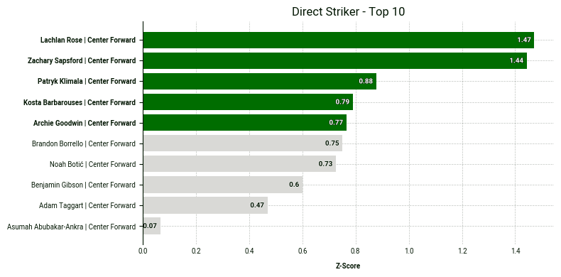
As we can see, Lachlan Rose and Zachary Sapsford stand out from the rest, indicating they rank particularly highly for the selected metrics. One of the benefits of using z-scores is that we can observe not just the ranking but the magnitude of differences between players.

Next, we are going to plot all three archetypes inside a scatter plot. Copy the code block below for the visualization: 

# --- 5. SCATTER PLOT USING df_scored ---
# Identify the Top 5 in Intensity and Explosivity to highlight and contrast them with volume using the bubble size.
top_5_direct_ids = df_scored.sort_values('Direct_Composite', ascending=False).head(5)['player_id'].tolist()
top_5_linkup_ids = df_scored.sort_values('Linkup_Composite', ascending=False).head(5)['player_id'].tolist()


highlight_players = list(set(top_5_direct_ids + top_5_linkup_ids))


fig, ax = scatter.plot_scatter(
   df=df_scored,
   x_metric='Direct_Composite',
   y_metric='Linkup_Composite',
   z_metric='Target_Composite',
   data_point_id='player_id',
   primary_highlight_group=highlight_players,
   data_point_label='player_short_name',
   x_label='Direct Striker (Z-Score)',
   y_label='Link-Up Striker (Z-Score)',
   z_label='Target Man (Z-Score)',


   primary_highlight_color='#006D00',
   plot_title='Direct vs. Link-Up vs Target',
)

‍

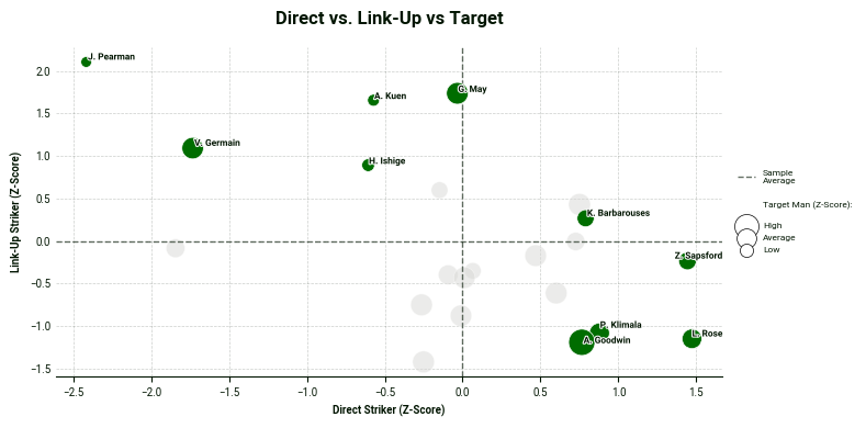
In the bottom-right corner, we find the most direct strikers, while the top-left corner is occupied by the link-up striker archetypes. Bubble size adds a third layer to the analysis, allowing us to evaluate the extent to which players from either cluster also display target man characteristics.

‍

5 - Visualizing Off-Ball Run Profiles

After placing the A-League strikers across the different archetypes, we can validate our results by examining their off-ball profiles using our bespoke radar from the SkillCorner Viz Library. The radar displays the number of runs a player makes for each specific run type, along with their corresponding percentile compared to our sample.

For example, let’s take a look at the off-ball profile of Valère Germain:

‍

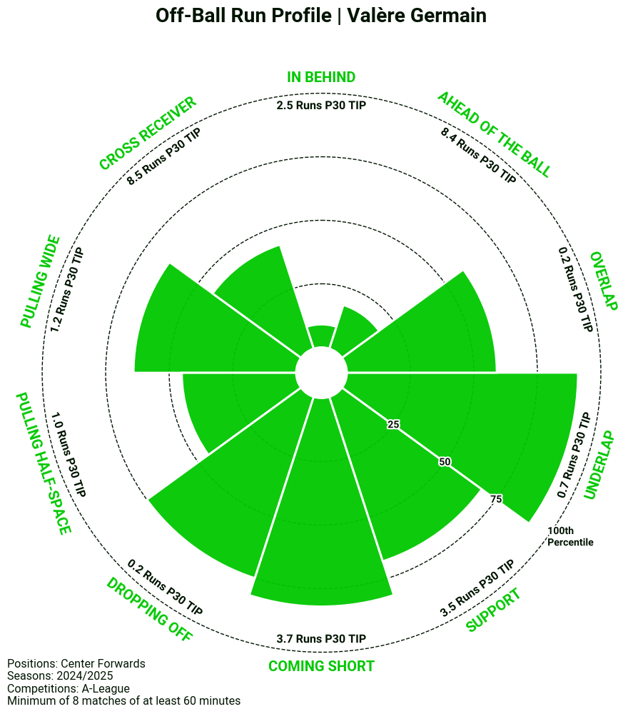
The radar aligns well with Germain’s archetype as a Link-Up Striker. This is evident in his 3.7 Coming Short Runs per 30 TIP, placing him above the 75th percentile.

Next, let’s examine Archie Goodwin’s radar, which is expected to score high on more traditional striker runs, such as Runs In Behind and Cross Receiver Runs as he ranks highly for both the Direct Striker Archetype and the Target Man Archetype. 

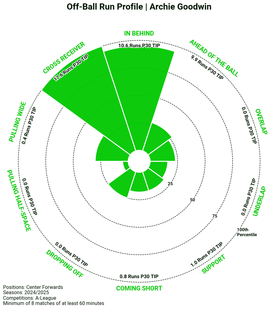
As expected, Goodwin ranks high for Runs In Behind, averaging 10.6 per 30 TIP. However, no one surpasses him in Cross Receiver run volume, where he averages 17.6 per 30 TIP. The 21-year-old was recently signed by Charlotte FC in the MLS, and has made an immediate impact by scoring three goals in his first five matches.

Below is the code for visualizing the off-ball runs: 

# Creating new dataframe, runs_df from initial df_filtered
runs_df = df_filtered


# Mapping Runs
RUNS = {'crossreceiverrun_count_p30tip': 'Cross Receiver',
       'behindrun_count_p30tip': ' In Behind',
       'aheadoftheballrun_count_p30tip': 'Ahead Of The Ball',
       'overlaprun_count_p30tip': 'Overlap',
       'underlaprun_count_p30tip': 'Underlap',
       'supportrun_count_p30tip': 'Support',
       'comingshortrun_count_p30tip': 'Coming Short',
       'droppingoffrun_count_p30tip': 'Dropping Off',
       'pullinghalfspacerun_count_p30tip': 'Pulling Half-Space',
       'pullingwiderun_count_p30tip': 'Pulling Wide'}


# Plot off-ball run radar for Nico Williams.
fig, ax = rad.plot_radar(runs_df[runs_df['position_group'] == 'Center Forward'],
                        data_point_id='player_name',
                        label='Archie Goodwin', # Which data_point_id to highlight. If you use a name, use player_name as data_point_id
                        plot_title='Off-Ball Run Profile | Archie Goodwin',
                        metrics=RUNS.keys(),
                        metric_labels=RUNS,
                        percentiles_precalculated=False, # Changed to False
                        suffix=' Runs P30 TIP',
                        filter_relevant=False, # Only color the run types that are important to you group like user group


                        # Create your own sample text
                        positions='Center Forwards',
                        matches=8,
                        minutes=60,
                        competitions='A-League',
                        seasons='2024/2025', add_sample_info=True)

6 - Go Further

In this installment, we’ve shown how you can merge different datasets and how Z-scores can be used to create archetypes. 

If you’d like to explore these composite models further or create your own archetypes for strikers or other position groups, you can find the full logic in our Google Colab notebook. Feel free to adapt the functions to build your own profiles. 

We always encourage you to share your work on social media. If you do, please reference SkillCorner as the source of the data and tag our relevant account on X/Twitter or LinkedIn.

‍